|
|
|
|
7.0. The Scope Program |
|
|
|
|
|
7.0. The Scope Program |
|
7.1.
Data Flow Diagram
7.1.1. Data Flow Paths
7.2 The Grid
7.3 The Traces
7.4. Storing and
Restoring the Pervious Position of the Main Frame
7.5. Setting-Up
RS232 Communications
7.6. Solving the
Flickering Problem
7.7. Creating
the Split Window View
7.8. Saving / Opening Scope Data
7.9. Copying the Scope Display to the Windows Clipboard
7.10. Exporting the Scope Display as a Bitmap (BMP) File
7.11. Owner Drawn Menus with Bitmaps
7.11.1. Integrating Brent Corkum's BCMenu Class with the Scope Program.
7.12. Windows 95/98 Compatibility Problem (scope v1/008a,
20/12/2001)
7.13. Windows XP Compatibility Problem (Scope v1.017a,
05/02/2002)
7.14. Additional Video Card Features That May Explain Low CPU
Usage.
This Windows based program, graphically displays waveforms without flicker, it has a good user interface that is easy to use, and directly communicates with the PIC. RS232 transport medium has been selected, this medium is easy to program, reliable and every PC comes with at least one RS232 port. But it is slow and will limit the maximum sampling rate in the real-time mode. Therefore it is important that the application is design to be flexible, as its probable that the program will be modified some time in the future for use with another medium (e.g. Parallel, USB, etc…).
The development of this program is not fully completed, but has progressed sufficiently to display real-time waveforms using various triggering methods, selectable time-base, selectable voltage scales, etc... Storage mode operation and direct control of the PIC has not been implemented yet, as well as some advantaged features like: streaming real-time data to disk, automatic frequency calculation, and the addition of user configurable virtual channels (e.g. VC1 = CH1 + CH2, VC2 = CH1 * CH2, etc…).
Please note that the full source code is contained on the attached CD ROM, as a full printout would require hundreds of pages. Allow important parts of the source code have been included in this chapter, along with a brief English description on how the code works.
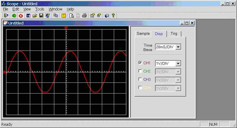
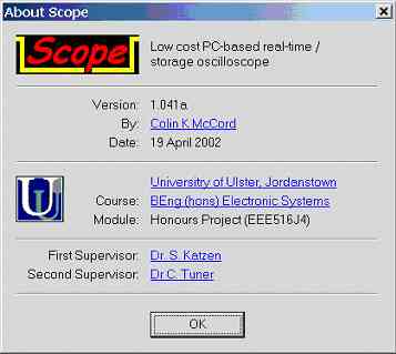
Figure 7.0a.
Screen dump of scope.exe (V1.041a, 19/04/2002)
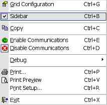
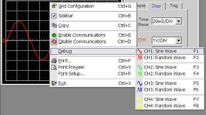
Notice that the display is split into two (see figure 7.0a), the left half displays the waveform and the right half contain the controls. The attached control dialog can be hidden; by right clicking on the waveform display and selecting [Sidebar] or by using the [View] menu (see Figure 7.0c).
|
Figure 7.0b. Right click menu |
At present four channels has been implemented. Data can be received in the real-time mode using the RS232 serial port. The real-time mode communications were first tested using the PIC simulator program, where sinewaves, squarewaves and random waves at variable frequencies and amplitudes were successfully sent to the scope program which correctly displayed the waveforms. (Desktop PC running scope.exe linked to Laptop running sim.exe via RS232 Null mode cable). Once the program was working on the simulator it was tested using a PIC sampling real waveforms, the scope program successfully displayed these waveform correctly, see chapter 11 (testing) for test results at various stages of development.
|
|
|
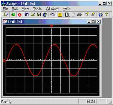
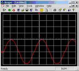
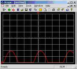
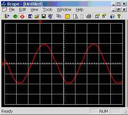
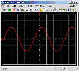
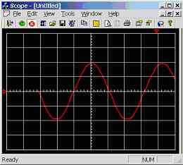
Notice the small red triangle at the left of the graphical display, this triangle shows the zero point of the displayed waveform. The user using the mouse can click on the triangle and drag it to a new position, hence changing the zero point (see figure 7.0e). Notice if the waveform is too high or too low for the display the top/bottom of the waveform will be cut off.
|
|
|
|
|
Figure 7.0e. Three screen dumps of scope.exe demonstrating the change of zero point |
||
Notice the small red triangle at the top of the graphical display, this triangle shows the offset position of the displayed waveform (middle of the screen represents zero offset). The user using the mouse can click on the triangle and drag it to a new position, hence changing the waveform offset (see figure 7.0f). Notice that if the waveform is offset to the right, it is possible to see data before the waveform triggered. This feature is mainly useful for helping in the measurement of waveform period time (use in calculation of frequency) where the waveform can be scrolled so that a peak is directly in line with a division line, making actuate measurement easy.
|
|
|
|
|
Figure 7.0f. Three screen dumps of scope.exe demonstrating the change of waveform offset |
||
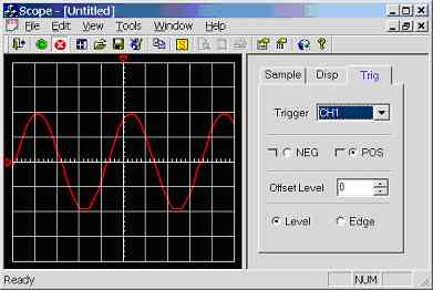
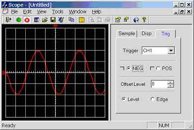
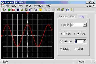
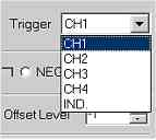
Also notice that the waveform triggers on a low to high edge (software trigger), this is user adjustable in the [Trig] tab of the controls dialog (see figure 7.0g). Notice the user has many options, level triggering means that a trigger occurs when the waveform rises from below to above the user configurable offset level for positive edged triggering and the waveform falls from above to below the user configurable offset level for negative edged triggering. Edge triggering means that the program detects the positive or negative edges of any waveform and at any voltage level, this guarantees that the waveform triggers without the need for user intervention, unlike level mode were the waveform must pass through the selected offset level.
|
|
|
|
|
|
|
|
|
|
Figure 7.0g. Six screen dumps of scope.exe demonstrating different trigger settings
|
|
|
|
The user can select which channel to trigger off: CH1, CH2, CH3, or CH4. Notice that there is another option called “IND.”, this means independent triggering, where each channel has its one unique trigger point. It is not sure how useful this feature is as generally for dual and quad trace operation waveforms are normally related is some way and timing analysis is normally required. It was decided to include this function for increased program flexibility as this allows for four unrelated waveforms to be monitored simultaneously on the same scope display. Besides it normal practice for commercial products to have useless features (Bells and Whistles) which will probably never be used in practice, but helps give their product an edge over the competition.
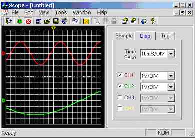
The [Disp] tab of the controls dialog can enable/disable channels simply by clicking the tick box beside each channel, change scope time-base and channel voltage scales (see figure 7.0h). Notice in figure 7.0h there are two enabled channels both of which have zero offset, hence the offset triangle for both channels are in exactly the same place (this is clear due to the colour of the triangle). This is not a problem (e.g. offset of both channels does not change if user clicks on the offset triangle) as channel 1 has absolute priority, hence only channel 1 offset will change separating the channel offsets. Note channel 2 has priority over channel 3 and channel 3 has priority over channel 4. A quick way of moving channel 4 offset for example, if all four channel are enabled and the offset of each is in the same place, is to temporarily disabled channels 1 to 3, move channel 4 offset and enable channels 1 to 3 again.
|
|
|
|
Figure 7.0h. Two screen dumps of scope.exe demonstrating different display settings |
|
|
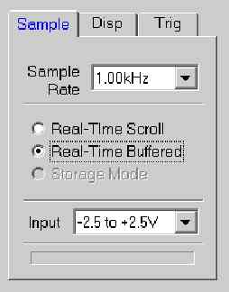
Figure 7.0i. [Sample] Tab of controls dialog |
The [Sample] tab of the controls dialog sets the sample rate, mode, and input range of the scope.
Note at present the ‘control’ communication protocol has not been implemented, hence the selected sample rate will not actually change the rate that the PIC is sampling. But it is important that the correct sample rate is selected as this is used in the calculation of the time-base, else the time-base selected in the [Disp] tab will be incorrect.
Note the input range is selected here, it was expected that this information is sent to the PIC to adjust the gain of the op-amps, but this has not been implement yet. Allow it is important that the correct input range is selected as this changes the binary representation of voltage (e.g. for a range of -2.5 to +2.5V, 0V = -2.5, 512 = 0V, 1024 = 2.5V and for a range of -5 to +5V, -5V = 0, 0V = 512, 5V = 1024).
Sampling mode is also selected here: Real-time scroll mode means that the waveform is sampled using the real-time mode, but stored onto the internal channel arrays in such away that the waveform appears to scroll across the screen (low frequencies only, e.g. useful for ECG monitor). Real-time buffered mode means that data is buffered before copying to the internal channels arrays and is triggered so that the waveform appears to be stable on the display (e.g. useful for periodical waveforms). Storage mode has not been implemented yet, recall that the PIC samples to RAM and then transmits the data to the PC in one large block with added CRC.
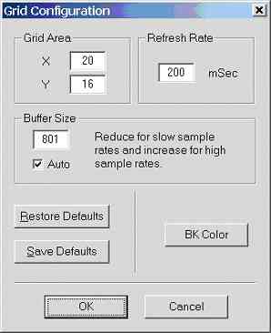
The grid configuration dialog box is shown in figure 7.0j; X specifies the number of horizontal squares (1 to 99), Y specifies the number of vertical squares (1 to 99). Note each square has 10 points; hence a maximum resolution of 999 by 999 is possible (assuming Window’s desktop resolution is larger than this). The default grid resolution is 10 x 8 (100 x 80), but 20 x 16 (200 x 160) is probably better suited for quad channel operation. Note the higher the grid resolution the more processor hungry the scope program becomes, hence extremely high resolutions are only recommend for high speed modern computers (e.g. 500MHz or above).
|
|
The refresh rate specifies the time in milliseconds between screen refreshes. For example 200 milliseconds is the default, that’s a refresh rate of 1/0.2 = 5 Hz. Some traditional analogue engineers who are use working with CRT displays will think that this refresh rate is too low and will result in the screen flickering. This is not the case, unlike CRT displays, the screen holds the current display contains between refreshes, and only redraws the changes made to the waveform when the screen is refreshed (perhaps this should have been called the ‘update rate’ rather than the ‘refresh rate’). The actual refresh rate is that specified by Windows, which for a modern PC is above 100Hz for a CRT display and 50/60Hz for a TFT display.
Note the lower this refresh rate (update rate) the more processor hungry the scope program becomes. A 200 milliseconds update rate will require a PC running at a minimum of 200MHz and at 50 milliseconds update rate will probably require a PC running at least 800MHz to run smoothly, depending on the selected grid resolution and type of video card in the system (hardware acceleration).
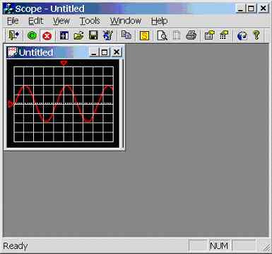
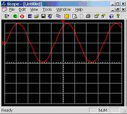
The scope program was designed so that multiple scope windows can be displayed; each one with its own selected channels enabled, impendent triggering, time-bases and scales. But it was not sure how useful this feature might be and it may have caused problems during the development process; hence it was considered this feature may be dropped on the finished application. Fortunately this did not cause as many problems as first expected and it was decided to keep this feature, as it may have some use for specialist applications and it’s another one of those features (“Bells and Whistles”) that sets this project apart from other similar products on the market.
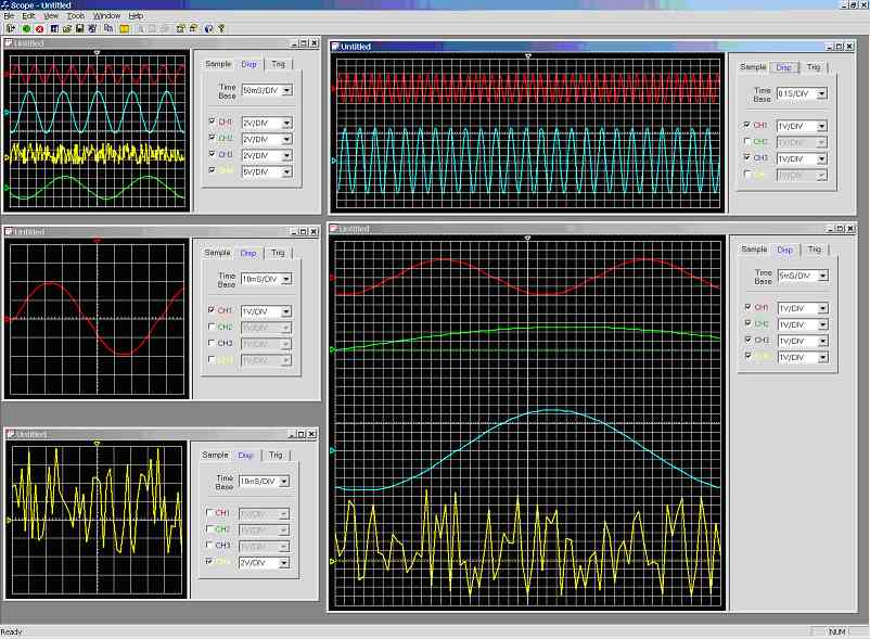
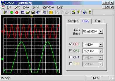
Figure 7.0k demonstrates the multiple windows feature, there are 5 views: The top left display, shows all four channels triggering on CH1 at a time-base of 50ms/DIV. The middle left display, shows CH1, with a time-base of 10ms/DIV. The bottom left display, shows CH4, with a 10ms/DIV time-base. The top right display shows CH1 and CH3 at a time-base of 0.1s/DIV. The bottom right display shows all four channels at an extremely high resolution at a time-base of 5ms/DIV and triggering off CH2. The only problem is that all scope windows have the same name “Untilled”, clearly this needs to be improved (e.g. “Untilled1”, “Untilled2”, etc…) as this is confusing to user, the reason for this is because the default automatic naming of the windows was overwritten so that filenames could be placed on the title bar. There is no limit on how many windows that can be opened simultaneously, perhaps until the computer runs out of memory, which on a modern PC could be 1000s of windows.
The scope program is also capable of exporting the scope display to the windows clipboard in the form of a bitmap and exporting the scope display to a bitmap file (*.bmp). The scope program also has its own file format (*.sdf) for saving and opening waveform data and scope settings. Note functionally for printing the scope display directly from the scope program is not fully complete, some additional work is required in this area.
|
|
|
|
|
The scope program is capable of generating software waveforms (see figure 7.0n), this was used to test the graphical display and triggering methods before the simulation program and PIC hardware was ready for testing. Note this menu will be removed in the final released version.
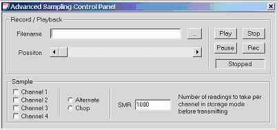
Another view exists (figure 7.0o), but has not been implement. It was expected that the user would enter a file name and press [Rec] to stream real-time data to disk and press [Play] to play back recorded real-time data.
When in pause mode the scroll bar labelled ‘position’ would have been used to manually scroll through the record data.
The tick boxes for channels 1 to 4 were to be used for telling the PIC which channel to sample. The reason why the enable / disable channels (in [Disp] tab) could not be used for this task is because multiple scope windows can be opened with different channels enable / disable hence a global set of enable / disable channels is required to specify which channels to sample.
The “Data Flow Diagram” shows how data flows between classes, but it does not give any details on the type of data being transferred. The following is detailed information about data flow in all numbered paths shown on the “Data Flow Diagram”: -
Path 1: CControlsP2 ßà CScopeDoc
|
int
m_TimeBaseSelection |
int m_nCH1_VOLTS |
int m_nCH2_VOLTS |
Path 2: CControlsP3 ßà CScopeDoc
|
int m_nTrigger |
int m_nTriggerOffsetLevel |
int m_nTriggerType |
Path 3: CMainFrame ßà CScopeApp
|
int m_nSampleMode |
int m_nBufferSize |
int m_nPOS |
Path 4: CScopeView ßà CGridConfigDlg
|
int x |
int y |
Path 5: ChildFrame ßà CScopeView
m_bShowPanel
Path 6: CGridConfigDlg ßà CScopeApp
m_nBufferSize
Path 7: CScopeView ß CScopeDoc
|
int m_TimeBaseSelection int m_nCH3_VOLTS |
int m_nCH1_VOLTS |
int m_nCH2_VOLTS
|
|
int m_nTrigger |
int
m_nTriggerOffsetLevel |
int
m_nTriggerFormat |
Path 8: CScopeView ß CScopeApp
|
int
m_nCH1Volt[10004] |
int m_nCH2Volt[10004] |
int m_nCH3Volt[10004] |
Path 9: CScopeDoc ßà *.sdf File
|
pApp->
m_nCH1Volt[10004] |
pApp->m_nCH2Volt[10004] |
pApp->m_nCH3Volt[10004] |
Path 10: CScopeDoc ßà CScopeApp
|
int
m_nCH1Volt[10004] |
int
m_nCH2Volt[10004] |
int
m_nCH3Volt[10004] |
|
Figure 7.2a. Grid layout |
The grid design is shown in figure 7.2a, there are 10 vertical and 10 horizontal points per square. The standard resolution has 10 horizontal squares and 8 vertical squares.
The grid is dynamic, flexible and is one of the key aspects of the scope program.
If the scope window is resized, the grid will automatically resize. The grid resolution is also user configurable; allow the resolution of each square is fixed the number of vertical and horizontal squares are user configurable.
There are two important arrays that must be filled after the scope window has been resized or the grid resolution has been changed (m_nGridY & m_nGridX), these arrays are used to access individual grid points.
For example the grid layout shown in figure 7.2a, has 100 horizontal (X) points and 80 vertical (Y) points. The scope window size is retrieved from the system and stored in variables m_nClientWidth and m_nClientHeight. m_nClientWidth is divided by 100 (X) and m_nClientHeight is divided by 80 (Y), this gives the gap in pixels between each grid point (note variables have been converted to floating point numbers for increased accuracy). The array m_nGridX[n] is filled by looping from n = 1 to n = 100 (X) and multiplying n by the gap between the horizontal grid points (convert back to data-type int after multiplication has taken place). The array m_nGridY[n] is filled by looping from n = 1 to n = 80 (Y) and multiplying n by the gap between the vertical grid points (convert back to data-type int after multiplication has taken place). Note there is also a configurable boarder offset (nBD) that must be included in the calculation
The two arrays can now be used as a coordinate system to access any part of the grid, for example the bottom left edge of the grid is at coordinate m_nGridX[1] by m_nGridY[1] and the top right edge of the grid is at coordinate m_nGridX[100] by m_nGridY[80]. Drawing of the grid and waveform traces is achieved using this coordinate system, the main advantage of this is that it does not matter what size the scope display is, the only thing that needs to change is the values contain within the coordinate arrays (extremely flexible).
Function PerpareGrid() fills the grid coordinate arrays: -
void CScopeView::PrepareGrid()
{
double fW, fH;
int n;
int nBD = 10; /* Border */
fW = ((double)(m_nClientWidth-(nBD*2)))/((double)x);
fH = ((double)(m_nClientHeight-(nBD*2)))/((double)y);
m_nGridX[0] =
nBD;
m_nGridY[0] = nBD;
for (n = 1; n <=x;n++)
{
m_nGridX[n] = ((int)(fW * n))+nBD;
}
for (n = 1; n <=y;n++)
{
m_nGridY[n] = ((int)(fH * n))+nBD;
}
}
Function OnDrawGrid() draws the grid using the grid coordinate system: -
void CScopeView::OnDrawGrid()
{
/*
----------------------------------------------------------
| Fuction: void CScopeView::OnDrawGrid() |
| Description: Draws grid in memory then updates display. |
| Return: Void. |
| Date: 09/12/2001 |
| Verison: 1.4 |
| By: Colin McCord |
----------------------------------------------------------- */
int n,i;
CClientDC dc(this);
CBitmap m_bitmapGrid, *m_bitmapOldGrid = NULL;
// if we
don't have one yet, set up a memory dc for the grid
if (m_dcGrid.GetSafeHdc() == NULL) m_dcGrid.CreateCompatibleDC(&dc);
m_bitmapGrid.CreateCompatibleBitmap(&dc, m_nClientWidth, m_nClientHeight);
m_bitmapOldGrid = m_dcGrid.SelectObject(&m_bitmapGrid);
m_bitmapOldGrid->DeleteObject(); // Make sure there is not a memory
leak
/* If the pen
is not setup, do not continue */
if(penGrid == NULL) return;
/* Select the
grid pen for use with the DC */
CPen* pOldPen = m_dcGrid.SelectObject(penGrid);
CBrush Brush;
Brush.CreateSolidBrush(m_ColorGridBackGround); // Grid Back
Colour
m_dcGrid.FillRect(&m_ClientRect,&Brush);
/* Draw
Border */
m_dcGrid.MoveTo(m_nGridX[0],m_nGridY[0]);
m_dcGrid.LineTo(m_nGridX[x],m_nGridY[0]);
m_dcGrid.LineTo(m_nGridX[x],m_nGridY[y]);
m_dcGrid.LineTo(m_nGridX[0],m_nGridY[y]);
m_dcGrid.LineTo(m_nGridX[0],m_nGridY[0]);
/* Draw V
Gray Lines */
for (n=10; n < x;n=n+10)
{
for(i = m_nGridY[0]; i<m_nGridY[y];i++)
m_dcGrid.SetPixel(m_nGridX[n],i,GRAY);
}
/* Draw H
grey line */
for (n=10; n < y; n=n+10)
{
for(i = m_nGridX[0]; i<m_nGridX[x];i++)
m_dcGrid.SetPixel(i,m_nGridY[n],GRAY);
}
/* Draw
Centre Axis */
m_dcGrid.MoveTo(m_nGridX[x/2],m_nGridY[0]);
m_dcGrid.LineTo(m_nGridX[x/2],m_nGridY[y]);
m_dcGrid.MoveTo(m_nGridX[0],m_nGridY[y/2]);
m_dcGrid.LineTo(m_nGridX[x],m_nGridY[y/2]);
/* Draw V
Ticks on H Centre */
for (n=2; n < x; n=n+2)
{
m_dcGrid.MoveTo(m_nGridX[n],m_nGridY[(y/2)-1]);
m_dcGrid.LineTo(m_nGridX[n],m_nGridY[(y/2)]);
}
/* Draw H
Ticks on V Center */
for (n=2; n < y; n=n+2)
{
m_dcGrid.MoveTo(m_nGridX[(x/2)],m_nGridY[n]);
m_dcGrid.LineTo(m_nGridX[(x/2)+1],m_nGridY[n]);
}
m_dcGrid.SelectObject(pOldPen);
/* Update Display */
Invalidate(TRUE);
}
The drawing of the traces looks extremely complex when looking at the big picture as channel offsets, zero positions, time-base, sample rate, triggering method, channel disabled/enabled and voltage scales all affect how the scope traces are drawn. Allow the basic principles behind the drawing of the waveforms are simple, so let’s try and describe how the waveform traces are drawn step-by-step.
There are four large arrays (one for each channel) in class CScopeApp: -
int m_nCH1Volt[10000];
// Voltage * 1000
int m_nCH2Volt[10000]; // Voltage * 1000
int m_nCH3Volt[10000]; // Voltage * 1000
int m_nCH4Volt[10000]; // Voltage * 1000
These arrays are global and can be accessed from any part of the program. Sampled readings for each channel are stored in these arrays; filled by the communication protocol, note the method used to fill these arrays is depended on which mode is selected e.g. for scroll mode every location is moved one placed to the left and the new reading is placed at the end of the array. Note the 10-bit ADC readings have already been converted into voltage depending on the selected input voltage range and multiplied by 1000 to increase resolution without having to use floating point numbers (e.g. for range -10 to 10V: -10V = -10000, 0V = 0 and 10V = 10000).
The basic principle is that the program continuously scans through these arrays updating the display at a user configurable refresh rate.
Software interrupt timer for redrawing traces: -
void
CScopeView::OnTimer(UINT nIDEvent)
{
if (nIDEvent
== nTimerRefresh)
{
KillTimer(nTimerRefresh);
Trigger(); /** Cal Trigger Points */
/* Set
scales */
m_nVPD_CH1 = pDoc->m_nCH1_VOLTS;
m_nVPD_CH2 = pDoc->m_nCH2_VOLTS;
m_nVPD_CH3 = pDoc->m_nCH3_VOLTS;
m_nVPD_CH4 = pDoc->m_nCH4_VOLTS;
/**
Draw Traces */
OnDrawCH1();
OnDrawCH2();
OnDrawCH3();
OnDrawCH4();
/*
Enable Timer again */
SetTimer(nTimerRefresh,m_nRefreshRate,NULL);
}
CView::OnTimer(nIDEvent);
}
The first thing to note is that the timer is stopped while executing the OnTimer() function and started again once the redraw is finished. The reason for this is to reduce the chance of the program locking up because of accumulating delays caused by the refresh rate selected by the user being shorter than the time required to redraw the display. In reality the true refresh rate is not the rate specified by the user, but the time taken to redraw the display plus the rate specified by the user, this insures that the program does not lockup especially when running on slow PCs (<200 MHz).
Function trigger() is called to find the trigger point for all channels, then the channel voltages scales are set to that selected by the combo box, then the channel traces are drawn.
This function calculates the trigger point: -
void CScopeView::Trigger()
{
int a = pDoc->m_nTriggerOffsetLevel;
/* CH1
Trigger */
for(int i = 1;i <= 1000;i++)
{
if (pDoc->m_nTriggerType == 0)
{
if(pDoc->m_nTriggerFormat == 1) a = pApp->m_nCH1Volt[i-1];
// Edge Triggered
/* trigger POS to NEG */
if (pApp->m_nCH1Volt[i] >= a && pApp->m_nCH1Volt[i+1] <
a)
{
m_nTriggerCH1 = i;
/* Disable trigger for scroll mode */
if (pApp->m_nSampleMode == 0) m_nTriggerCH1 = 0; // disbale trigger
i = 1001;
break;
}
}
else
{
if(pDoc->m_nTriggerFormat == 1) a = pApp->m_nCH1Volt[i-1];
// Edge Triggered
/* trigger NEG to POS */
if (pApp->m_nCH1Volt[i] <= a && pApp->m_nCH1Volt[i+1] >
a)
{
m_nTriggerCH1 = i;
/* Disable trigger for scroll mode */
if (pApp->m_nSampleMode == 0) m_nTriggerCH1 = 0;
// disbale trigger
i = 1001;
break;
}
}
}
...
NOTE channel 2-4 trigger point calculated the same way as channel 1
...
switch (pDoc->m_nTrigger)
{
case
0: // trig on CH1
m_nTriggerCH2 = m_nTriggerCH1;
m_nTriggerCH3 = m_nTriggerCH1;
m_nTriggerCH4 = m_nTriggerCH1;
break;
case
1: // trig on CH2
m_nTriggerCH1 = m_nTriggerCH2;
m_nTriggerCH3 = m_nTriggerCH2;
m_nTriggerCH4 = m_nTriggerCH2;
break;
case
2: // trig on CH3
m_nTriggerCH1 = m_nTriggerCH3;
m_nTriggerCH2 = m_nTriggerCH3;
m_nTriggerCH4 = m_nTriggerCH3;
break;
case
3: // trig on CH4
m_nTriggerCH1 = m_nTriggerCH4;
m_nTriggerCH2 = m_nTriggerCH4;
m_nTriggerCH3 = m_nTriggerCH4;
break;
}
}
Detection of the trigger point is simple; basically the program scans the array and looks for a high-to-low or a low-to-high edge. The location of which is stored (m_nTriggerCH1..4), this producer is carried out for all four channels. If a specific channel is selected as the trigger, the trigger points of the other channels are made equal to the trigger point of the selected channel.
A memory DCs and pen is required for each trace: -
CPen* penCH1;
CDC m_dcCH1;
CDC m_dcCH2;
CPen* penCH2;
CDC m_dcCH3;
CPen* penCH3;
CDC m_dcCH4;
CPen* penCH4;
Variables are initialised in the CScopeView constructor: -
CScopeView::CScopeView()
{
m_bitmapCH1 = NULL;
m_bitmapCH2 = NULL;
m_bitmapCH3 = NULL;
m_bitmapCH4 = NULL;
m_nClientHeight= 0;
m_nClientWidth = 0;
x = 100;
y = 80;
/** Zero
Point Positions **/
m_nCH1POS = 40;
m_nCH2POS = 20;
m_nCH3POS = 50;
m_nCH4POS = 60
}
Refresh timer, trace colours, grid colour and the grid background colour are setup here: -
This function is called when a channel voltage scale combo box is changed: -
...
Channel 2-4
done in exactly the same way as channel 1
...
...
Channels 2-4 prepared in exactly the same way as channel 1
...
}
The code marked in red is the actual drawing of the waveform; basically the array is scanned and drawn to the channel DC (m_dcCH1) using the grid coordinate arrays m_nGridX[] and m_nGridY[] . The code looks more complex because of the following variables: m_nTriggerCH1 specifies the array trigger offset, m_nCH1_Offset specifies the channel offset, m_Skip specifies the number of array locations to skip to achieve the required time-base, m_MUX specifies the number of array location to duplicate to achieve the required time-base, and m_nVPD_CH1 sets the voltage scale. Note drawing of the zero point and offset arrows are also drawn in this function and all four channels are drawn in exactly the same way. This function is called by the system when the scope display is resized: -
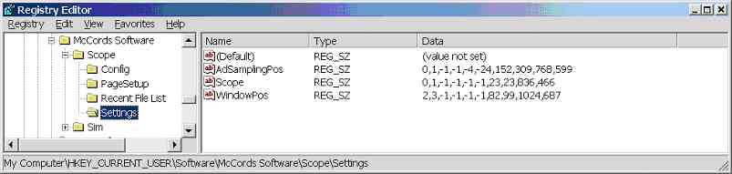 Figure 7.4a.
Screen dump of window registry showing where the window position is stored
Figure 7.4a.
Screen dump of window registry showing where the window position is stored
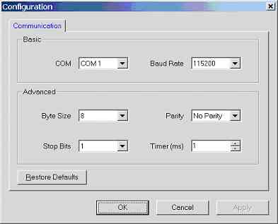
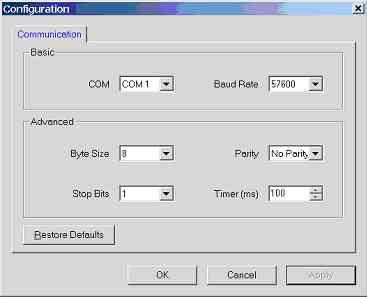 Figure 7.5a.
Screen dump of the configuration dialog box
Figure 7.5a.
Screen dump of the configuration dialog box
|
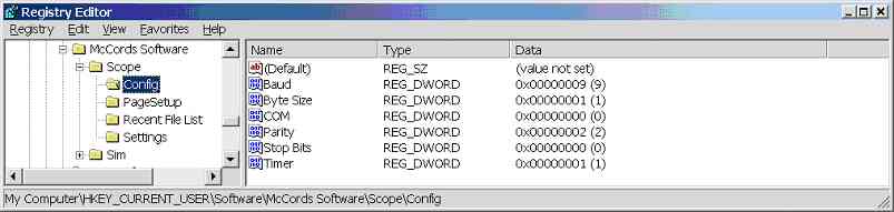 Figure 7.5b.
Screen dump of windows registry
Figure 7.5b.
Screen dump of windows registry
This Web Page was last updated on Friday June 28, 2002
Home About me National Record Of Achievement Hobbies / Interests Guest Book Contact Me Links Snooker Amateur Radio Site Map
|
© 2002 Designed by Colin K McCord |
|
This website is best viewed by Microsoft Internet Explorer 6.0 at a resolution of 1024 x 768